Navigating the valuation of complex debt instruments

Corporations are increasingly raising capital through debt instruments. Against the backdrop of rising debt financing, debt valuations are gaining traction due to financial reporting requirements and other purposes. The appraiser needs to be acquainted with the nuances of the valuation of debt securities. This article intends to cover the gamut of debt instruments and their valuation, including types and key characteristics of debt instruments, aspects to consider when valuing the debt instruments, major valuation methodologies and practical examples and case studies. Further, there is a higher emphasis on methods and case studies covering complex and convertible debt securities.

Background

All entities are capitalized with debt and equity. The nature and mix of debt and equity securities that comprise an entity’s capital structure, and its decision about the types of securities to issue when raising capital depends on the stage of the entity’s life cycle, the cost of capital, the need to comply with regulatory capital requirements, debt covenants and financial reporting implications. The complexity of the terms and characteristics of debt securities is influenced by factors such as the entity’s size, age, and/ or creditworthiness.[1]

Overview of debt instruments

A debt instrument is a fixed-income asset that legally obligates the debtor to provide the lender interest and principal payments.[2] Types of debt instruments include secured and unsecured notes, debentures, bonds, mortgage notes, and equipment obligations.[3] The key characteristics of debt instruments are:[4]

It creates a contractual obligation to repay the creditor.
It is senior to equity instruments and hence is less risky than equity.
Debt obligations include both principal and interest payments.
Interest payments are generally tax-deductible to the issuer.
Interest payment may be in cash, paid-in-kind (“PIK”), or both.
The interest rate could be fixed or floating, and the debt may have an interest rate cap, floor, or both.
Some debts are amortized, and some have bullet payments at maturity.
Debt could be traded or non-traded.
Terms are outlined in the loan agreements or bond indentures.

Types of debt instruments

Straight debt

Straight debt refers to a type of debt that does not have any options attached to it. It is a simple borrowing in which the issuer promises to pay back the principal amount at a specific maturity date along with periodic interest payments.[5]

Convertible debt

Convertible debt is a complex hybrid instrument with an option to either convert or redeem, with these choices being mutually exclusive and which cannot exist independently of one another. The holder cannot exercise the option to convert unless they forgo the redemption right or vice versa.[6]

Both convertible and non-convertible debt may have features such as callability and put-ability. Callability is the ability of the issuer to call a convertible debt at a predetermined price, and put-ability is the debtholder’s right to redeem convertible debt at a predetermined price.[7]

Convertible debt instruments continue to remain popular due to cheaper financing than straight debt. Convertible debt generally pays a below-market interest rate to investors compared to straight debt with similar risk/rating in exchange for providing them an embedded call option to convert the debt instrument into the issuer’s equity at the specified conversion terms.[8] The conversion terms could include valuation caps and discounts, as the section below explains.

Simple Agreement for Future Equity (“SAFE”)

[9]

Y Combinator, a technology startup accelerator, introduced the concept of SAFE after finding that founders of pre-revenue companies faced difficulty raising their first round of funding. SAFEs are a form of convertible financing, but differ from convertible debt in two ways:

SAFEs do not have maturity dates.
SAFEs do not have an interest rate.

SAFE investors have the option to convert SAFE into equity at the issuer’s next equity financing round or liquidity event. The conversion terms are usually determined by a valuation cap or a discount rate. The triggering events for SAFE notes are financing, liquidity (IPO, M&A, SPAC) and dissolution.

The terms of the conversion are usually determined by either a valuation cap or a discount rate:

Valuation cap: This is the maximum price at which a SAFE converts. The lower the cap, the better for investors because they will be able to convert SAFEs into a greater number of shares.
Discount rate: This is the discount to the priced round that SAFE holders get when they convert. The discount reduces the valuation used to calculate investors’ shares, allowing them to convert into more equity.

Debt Covenants

[10]

Debt covenants are clauses in the loan agreement with which the borrower guarantees to comply. Examples of debt covenants include maintaining key financial ratios such as equity, leverage or interest coverage ratios, meeting or exceeding key financial metrics such as predefined revenue or profitability targets, and clauses such as material adverse change. When a company breaches a covenant on or before specified dates, the outstanding debt liability may become repayable on demand (a put option) and/or the terms of the debt may become more punitive, for instance, a higher interest rate. This put option may be treated as an embedded derivative and may need to be valued under ASC 815.

U.S. Fixed Income Market

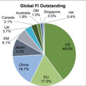
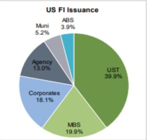
The U.S. fixed income markets are the largest in the world at $52.0 trillion (as of F.Y. 2022), comprising 40.0% of the global market. This is 2.3x the next largest market, the E.U. U.S. market share has averaged 38.1% over the last 10 years, troughing at 37.5% in 2013 and peaking at 40.0% in 2022. Within the U.S. fixed income market, treasury issuance (“UST”) is predominant, followed by corporate debt issuance.[11]

In recent months, U.S. borrowers have turned to convertible bonds as mainstream debt and equity markets have stumbled in the face of inflationary and interest rate headwinds. Combined leveraged loan and high-yield bond deal volume in the U.S. was down 26.0% in Q1 2023, year-on-year, reaching 396 deals. Leveraged finance value was similarly down by 24.0% year-on-year, reaching $240.5 billion.[12]

As a result, U.S. convertible bonds have surged as the pool of available liquidity has contracted. According to Dealogic, a financial markets platform offering integrated content, analytics, and technology, the overall issuance of U.S. convertible bonds was just under $12.0 billion in Q1 2023, nearly double the $6.2 billion recorded in Q1 2022.[13]

Convertible bonds have traditionally been issued by growth-oriented companies that are either not yet mature, or profitable enough to tap mainstream debt markets, or do not have high market capitalizations to raise sufficient capital from equity offerings. In most years, a significant proportion of convertible bond issuances involve borrowers who do not have credit ratings.[14] Meanwhile, investment-grade issuers that can access standard bond and loan markets have historically avoided convertible bonds because the structures raise the risk of issuing shares at a discount and diluting existing shareholders. However, in 2023, several investment grade and high-yield issuers have entered the convertible bond market to take advantage of the lower interest rates.[15]

Changes to U.S. accounting rules have also helped draw more issuers to the convertible bond space as accounting for convertible bonds has been simplified. Rules mandating that companies issuing convertible bonds add a hypothetical interest expense on the bonds in their accounts (thereby increasing the cost of issuance) have also been dropped. These changes to the accounting treatment have given convertible bond issuance an additional boost.[16]

Debt Valuation

In general, debt valuation is required for the following purposes:

Financial reporting (ASC 815, ASC 480, ASC 470, ASC 805)
Gift & estate tax planning
Other purposes, such as litigation

Considerations for Debt Valuations

Synthetic Credit Rating

Many small firms and private businesses are not rated by credit rating agencies. Hence, synthetic credit rating is used to determine the discount rate for their debt.
To make this assessment, we consider comparable publicly listed rated firms, followed by calculating key financial and leverage ratios and doing a DuPont analysis for both the company and the comparable companies.
The base credit rating is determined based on the comparable public companies. This base rating is then adjusted to reflect the subject company’s relative position against identified comparable public companies.
The applicable discount rate is determined based on the concluded credit rating.

Calibration and Recalibration

AICPA Guidance in the “Valuation of Portfolio Company Investments of Venture Capital and Private Equity Funds and Other Investment Companies” defines calibration as: “The process of using observed transactions in the portfolio company’s own instruments, especially the transaction in which the fund entered a position, to ensure that the valuation techniques that will be employed to value the portfolio company investment on subsequent measurement dates begin with assumptions that are consistent with the original observed transaction as well as any more recent observed transactions in the instruments issued by the portfolio company.”[17]
After determining the synthetic credit rating and the applicable discount rate, this rate will need to be calibrated on subsequent reporting dates to reflect the market conditions and the company-specific considerations.

Valuation Methodology

Discounted Cash Flow (“DCF”) Method

In this method, the value of the convertible debt is estimated as the present value of the contractual cash flows that debtholders receive over its term, discounted to the present value at the discount rate reflecting the underlying risk. The cash flows typically include principal and interest payments, upfront fees, and final closing fees, along with adjustments for warrant coverage, prepayments, etc. Furthermore, on the debt issuance date, typically, the discount rate estimated is the IRR, i.e., the rate that would result in the present value of the debt’s cash flows being equal to its principal amount. This is based on the consideration that the debt issuance terms, especially the interest rate, are at the market as of its issuance date. As noted above, the discount rate may be modified on subsequent measurement dates to reflect changes in market yields and the company’s performance.

Black Scholes Model (“BSM”)

The BSM model is a pricing model for financial instruments. The BSM model is used to determine the fair prices of stock options (put/call) based on six variables: volatility, dividends, underlying stock price, strike price, time, and the risk-free rate. It can also be used to value the conversion option embedded in convertible debt.

Binomial Option Pricing Model

The Binomial Option Pricing Model is a mathematical technique that estimates the value of an option by simulating potential price movements of the underlying asset. It uses a decision-tree approach to determine the option’s value at each possible future point in time.

Three key components of the Binomial Option Pricing Model are binomial tree, risk-neutral probabilities, and backward induction. The binomial tree represents the possible price movements of the underlying asset, risk-neutral probabilities used to calculate expected payoffs, discount rate, and backward induction that calculates the option’s value at each node. The Binomial Option Pricing Model applies to various types of options, including European, American, and exotic options.

Steps in the Binomial Option Pricing Model:

Building the Binomial Tree: The binomial tree is a visual representation of the possible underlying asset value movements over time. It is constructed by dividing the time to expiration into equal intervals and calculating the possible asset value at each node.
Option Valuation at Maturity: At the end of the binomial tree, the option’s value is determined by comparing its strike price to the underlying asset’s value. This comparison results in either a positive payoff or zero, depending on whether the option is in or out of the money.
Risk Neutral Probabilities: Risk-neutral probabilities are used to calculate the expected payoffs at each node in the tree. These probabilities are calculated based on the risk-free interest rate, asset value movements, and time between steps.
Discount Rate: For discounting purposes, the Tsiveriotis-Fernandes Model suggests classifying the value of the convertible debt into debt and equity components. The debt portion is discounted with a risky yield (in line with the creditworthiness of the bonds and the implied yield), while the equity portion is discounted using the risk-free rate.
Backward Induction: Backward induction is the process of working backward through the binomial tree to determine the debtholder’s payoff at each node. The expected payoffs at each node are discounted to the present, resulting in the debt’s current value.

For convertible debt valuations, the binomial model typically has four trees:[18]

Stock Price Tree;
Conversion Probability Tree;
Discount Rate Tree; and
Value/Payoff Tree.

(1) Stock Price Tree:

The first step in the binomial option pricing model is to determine the expected up and down movement of the stock price at each node as well as the probability of the up and down moves. The up/down factors are the factors by which the asset price will rise/fall in any given time step (with the down factor a reciprocal of the up factor), and are a function of the volatility and the term (including the number of nodes). The up/down probabilities are a function of volatility, risk-free rate and the term. Based on these factors, the stock price at each node is determined.

(2) Conversion Probability Tree

On the maturity/conversion date, for all nodes corresponding to that date, a comparison is done for whether it is beneficial for the debtholder to convert to equity or get repayment. If, for a particular node, the value to the debtholder on conversion based on the stock price as determined in the Stock Price Tree above is greater than the repayment amount the debtholder would receive when the debt matures, the debtholder would elect to convert in that node. Otherwise, the debtholder would opt to receive the principal and coupon payment in that node. As we move from right (maturity) to left (valuation date (“V.D.”)) of this tree, the following equation is used to determine conversion probability at each node:

q_n_,_i = (q_n₊₁,_i₊₁)(P) + (q_n₊₁,_i)(1 – P), where

q_n_,_i₌the conversion probability of the node being calculated

q_n₊₁,_i_{+1 =}the conversion probability of the up node to the right of the node being calculated

q_n₊₁,_i₌the conversion probability of the down node to the right of the node being calculated

P = up probability

(3) Discount Rate Tree

If the convertible debt is out-of-the-money, i.e., if the debtholder receives principal and coupon, the cash flows should be discounted at the risk-free rate plus a credit spread.

If the convertible debt is in the money, the future cash flows would be discounted at the risk-free rate since the risk is already reflected in the volatility because the conversion feature is priced as if it were a stock option.

For constructing credit-adjusted spread tree, the following equation is applied.

r_n_,_i = (q_n,_i r) + (1-q_n,_i)(r + k)

r_n_,_i₌the discount rate of the node being calculated

q_n_,_i₌the conversion probability corresponding to the node being calculated.

r = risk-free rate corresponding to the term of the convertible note.

k = the credit spread of the convertible note.

(4) Value/Payoff Tree

For constructing a convertible debt value tree, the following equation is applied:

p_{n,i =}Max [s_n,im, (Pp_{n+1 ,i}e^-r_n+1,^step) + ((1-P)p_{n-1, i}e^-r_n-1,^step)

p_n,i = value of the convertible note at the node being calculated

s_n,i = value of the stock at the node being calculated

m = the conversion ratio

P = the risk-neutral up probability

p_{n+1 ,i} = value of the convertible note at the up node to the right of the node being calculated

r_{n+1 ,i} = the discount rate at the up node to the right of the node being calculated

p_{n-1 ,i} = value of the convertible note at the down node to the right of the node being calculated

r_{n-1 ,i} = the discount rate at the down node to the right of the node being calculated

e= 2.71828, the base of the natural log function

step = the time until maturity of note divided by the number of steps

The value of the convertible debt at time 0, by following this process, would result in the value of convertible notes as of the V.D.

Monte Carlo Simulation (“MCS”)

This method involves running a large number of simulations using random number generators to address changes in key variables, which are intended to mimic what could happen with respect to the asset/security over time. Given a large enough sample size of simulations, the observations of the distributions of outcomes and various measures for central tendency approach the metrics that represent the core attributes of the security. MCS is a method by which many possible value outcomes are evaluated to establish the expected value of a security or an asset. This methodology allows the modelling of securities with complex terms, where path dependency, floors, caps, triggers, IPO, changes of , and next financing round provisions can be explicitly factored into the model construct.

Illustrative Case Studies

Case #1

Scope: Valuation of convertible notes issued by medical solutions provider

Background: The client required the valuation of convertible notes for sale to related parties. The valuation was required for multiple notes with different issuance dates. We performed initial measurement (calibration) and subsequent measurements for these notes.

All notes had identical terms, though issued at different dates. The notes were convertible at a discount to the company’s common stock or payable (principal + accrued interest) at the option of the noteholders at the earlier of (i) change of control event, or (ii) maturity date.

Further, a change of control event before the maturity date of these notes was unlikely.

Methodology: DCF for straight debt and BSM for conversion option.

Valuation Description:

Initial Measurement/Calibration – Issuance Date

Conversion Option

We calculated the value of the note’s option component using BSM and considered the following inputs:

Stock price: Per share value of the subject company’s common stock value was considered from the IRC 409A valuation in proximity to the note issuance date.
Strike price: The price at which the principal plus accrued interest converts to the subject company’s common stock.
Time to maturity (“Term”): Based on the note agreement.
Risk-free rate: The yield on U.S. treasuries corresponding to the Term.
Volatility: Based on the comparable guideline public companies corresponding to the Term.

Straight Debt Component

We prepared a DCF analysis with cash flows based on the terms outlined in the note agreement and backsolved for the yield, such that the present value of the cash flows equates to the note principal less the option value as estimated above.
After that, we calculated the spread over the treasury rate by deducting the treasury benchmark rate corresponding to the Term from the implied yield calculated above.
We observed that the spread was at the higher end of the market yields, indicating an implied credit rating of CCC and lower.
Then, we examined the option-adjusted spread (“OAS”) of CCC and lower-rated bond indices as of the note issuance date.
Finally, we calculated the company-specific risk premium as the difference between the spread over the treasury bond (point 2 above) and the median market spread for CCC and lower-rated bonds (point 4 above).

Subsequent Measurement Date

As of the subsequent measurement date (“V.D.”), we prepared a DCF analysis to determine cash flows for the straight debt component from the V.D. to the note maturity date.
Since Management indicated no change in business outlook since the initial measurement date, we considered the credit rating as unchanged between the initial measurement date and the V.D. Accordingly, we calculated the applicable discount rate as the sum of (i) the median OAS of CCC and below-rated bond indices as of the V.D., (ii) the company-specific risk premium, and (iii) the treasury rate corresponding to the remaining term of the note.
We calculated the value of the straight debt component using the DCF based on the discount rate determined above.
We calculated the value of the option component based on the inputs mentioned in the “Issuance Date” section above. However, the term considered was from the V.D. through the maturity date, with the volatility and the risk-free rate corresponding to this term.
The fair value of the note was the sum of the value of the straight debt portion and the value of the option component.

Case #2

Scope: Valuation of convertible notes issued by a biotechnology company

Background:

The principal and the accrued interest on the notes would convert to the shares of the subject company under various scenarios based on the review of the terms outlined in the convertible note agreement:

IPO/SPAC: Conversion at SPAC pre-money, at a discount.
Next Equity Financing (“NEF”): Conversion at the lower of the valuation cap or a discount to the original issue price (“OIP”) of the NEF.
Corporate Transaction (“M&A”): Conversion at the lower of per unit M&A consideration or per unit value based on the valuation cap.
Maturity: At the option of the noteholder, repayment of debt or conversion at valuation cap.

Methodology: Scenario Analysis with MCS

Valuation Description: Following scenarios were considered, and payoff under each scenario was weighted based on the probability of the scenarios occurring.

SPAC/IPO:
Since Management was expecting a SPAC/IPO with a near-term filing, the pre-money valuation based on the SPAC/IPO agreement was considered, based on which the per-share value of the company’s common stock was determined and was adjusted for discount as noted above.
Then, the resultant shares were multiplied by the per unit value at SPAC to determine the payoff for notes.
NEF:
We determined the market value of invested capital (“MVIC”) as of the V.D. as the sum of (a) the equity value of the subject company based on the risk-adjusted net present value method, and (b) the convertible note balance.
We then used the MVIC as calculated above as the base and simulated the MVIC as of the NEF date utilizing the Geometric Brownian Motion (“GBM”) framework within MCS and subtracted the value of debt (converted principal and interest) as of the NEF date to estimate the company’s equity value, i.e., pre-money for the NEF, and subsequently, the implied OIP for the NEF.
As noted above, we calculated the per unit value on conversion to noteholders as the lesser of (a) discount to the OIP, or (b) per unit value derived based on the valuation cap.
Based on the above-determined conversion price and the OIP per unit, the payoff to the notes at conversion was determined.
M&A
For M&A, we simulated the equity value up to the expected M&A date and adjusted it for control premium to determine the M&A consideration. We then considered the conversion of the notes at the lower of the valuation cap and M&A consideration, as noted above.
Using the above-determined conversion price and the value per unit based on the M&A consideration, the payoff to the notes at conversion was determined.
Maturity
- As noted above, we simulated the equity value up to the maturity date and then calculated the value per unit based on this equity value. We also considered the conversion of the notes based on the valuation cap, as noted above.
- Using the above-determined conversion price and the value per unit based on the equity value at maturity, the payoff to the notes at conversion was determined. Further, it was determined whether the debt repayment or conversion would be beneficial for the noteholders.
Discounting
Since the company was an early-stage biotechnology company with no product revenue, it was considered comparable to CCC-rated public companies.
The selected discount rate was within the range of rate observed for CCC-rated loans and was consistent with the company’s stage of development.

Case #3

Scope: Valuation of SAFEs issued by nuclear power generation company

Background: The client issued notes in multiple closings at different valuation caps.

Since these were SAFE notes, they were not subject to interest or maturity dates.
The principal amount would convert to the shares of the subject company or receive a cash payment under various scenarios based on the terms outlined in the SAFE agreement.
NEF: Conversion at the lower of the valuation cap or the OIP of the NEF.
Liquidity Event:
Noteholders receive greater of (i) the purchase amount (the “cash-out”) or (ii) the amount payable on the number of common shares equal to the purchase amount divided by the liquidity price.
Liquidity price was defined as the valuation cap divided by liquidity capitalization as defined in the agreement.
Liquidity events include IPO, SPAC, and M&A.
Dissolution: In case of dissolution, the holder would receive the portion of proceeds equal to the cash-out amount.

Methodology: MCS

Valuation:

The following inputs were considered for the purposes of the analysis:
Financing lock-out period (the time period up to which the company does not expect to raise financing).
NEF raise amount and pre-money valuation of the subject company as of the NEF date.
Probabilities of NEF and M&A.
M&A and IPO restriction periods (the time period up to which the company does not expect M&A and IPO/SPAC).
IPO and SPAC equity value threshold (the scenarios will be triggered only when threshold equity values are attained).
Dissolution (the company did not expect dissolution up to a certain period, given its ability to raise financing and sustain operations).
Considering the above inputs, the following steps were performed:
We arrived at MVIC as of the V.D. by utilizing the adjusted equity value method.
The adjusted equity value method involved considering equity value as of the prior 409a V.D. and applying percentage change based on observed market capitalization change of guideline public companies and company-specific developments.
We considered the MVIC as of the V.D. as a starting point and simulated it using GBM over a five-year period, the maximum period by which the SAFE notes are expected to convert or be paid off.
We also built an allocation waterfall as the company had a complex capital structure with common and preferred shares. The equity value determined for each iteration was allocated between various classes of securities, including SAFE.
At each iteration, the payoff to SAFE holders under each scenario mentioned in the Background above was calculated and adjusted for probability of occurrence. Also, the time of occurrence of these scenarios was calculated.
The mean results of the payoff and the mean time duration for each scenario were considered based on simulations. The implied yield was calculated such that the probability-weighted value of payoffs for the SAFE equates to the original investment value as the SAFEs were issued close to the V.D.
In subsequent valuation, which was at a V.D. six months after the initial measurement, a similar model framework with updated assumptions was considered to determine payoffs for the mentioned events.
Also, in the subsequent valuation, for the purposes of yield calibration, we measured the change in the observed market yield for a bond universe with a similar risk profile and considered company-level developments to determine the discount rate to discount the probability-adjusted payoffs for each scenario and, determine the fair value of the SAFEs.

Case #4

Scope: Valuation of convertible notes issued by medical device company

Background: The company issued two sets of notes with similar features except interest rate. While one note had a fixed coupon, the other had a variable rate linked to SOFR.

The notes were convertible at any time at the holder’s option, subject to a cap of a certain percentage of the fully diluted share count of the subject company (“Beneficial Ownership Cap”).
The noteholder had the option to demand repayment of outstanding principal and accrued interest in case of a change of control or a default event.
The notes had embedded conversion features and embedded redemption features. There was a de minimis probability of redemption and a change of control event; hence, these scenarios were not explicitly modeled.

Methodology: Binomial Option Pricing Method

Valuation:

We considered following inputs for the purposes of this analysis: Share price, Time to liquidity (“Term”), Equity volatility, Risk-free rate, Note conversion price, Coupon rate, Bond yield, and Discount for lack of marketability.
The subject company was publicly traded, so the starting share price was as of the V.D. was available. However, since the fully dilutive common stock held by the holder was higher than the average daily traded volume of the stock, a block discount was applied to the stock price as of the V.D. Then, the stock prices at subsequent nodes were estimated with an up and down factor, which were determined as noted in the Binomial Option Pricing Model section.
The Term was considered as the difference between the V.D. and the notes’ maturity date.
After that, we constructed the following trees and determined the conversion value using a backward induction process. The steps related to each are outlined in the Binomial Option Pricing Model section.
Share Price: Determined the share price at each node as described in the point above;
Conversion probability: At the maturity date, we determined the conversion or repayment based on the payoff to noteholders based on the share price(s) at the node(s). We then determined the conversion probabilities at the previous nodes using backward induction and used these probabilities to determine the probability-adjusted payoff and discount rate at each of the nodes;
- Probability-adjusted discounting factor: The discount factor to present value the payoff was probability-adjusted, as discussed above. Per the Tsiveriotis-Fernandes Model, the bond yield and the risk-free rate were considered as the discount rates for the debt portion and the equity portion, respectively, and
Payoff to the convertible notes: Based on the points above and through the process of backward induction, the payoff to the convertible notes at each node was determined.
Bond yields were estimated based on synthetic credit rating analysis, estimated by comparing certain financial ratios and metrics of the subject company, including leverage ratios (debt ratio, debt to equity ratio, and interest coverage ratio), the outcome of DuPont Analysis, etc. to those of comparable issuers which with publicly available credit ratings from Standard & Poor’s (“S&P”).
Based on the above analysis, we considered yield for CCC-rated bonds based on synthetic credit rating.